Difference Between Correlation and Regression

Correlation and regression are two important concepts in statistics that aim to explore the interdependence of particular phenomena. Both are generally used during data analysis, helping to understand the influence of one factor on another. Such techniques have found applications in many areas including management, finance, and the sciences, where information-based decisions are important.

While correlation explains how closely two variables are related, regression contains a predictive aspect projecting future values of a dependent variable by employing the independent variable. But you can find notable differences between these two types of analysis. Also, both of these techniques are necessary for you to analyse different patterns and trends in the given dataset.

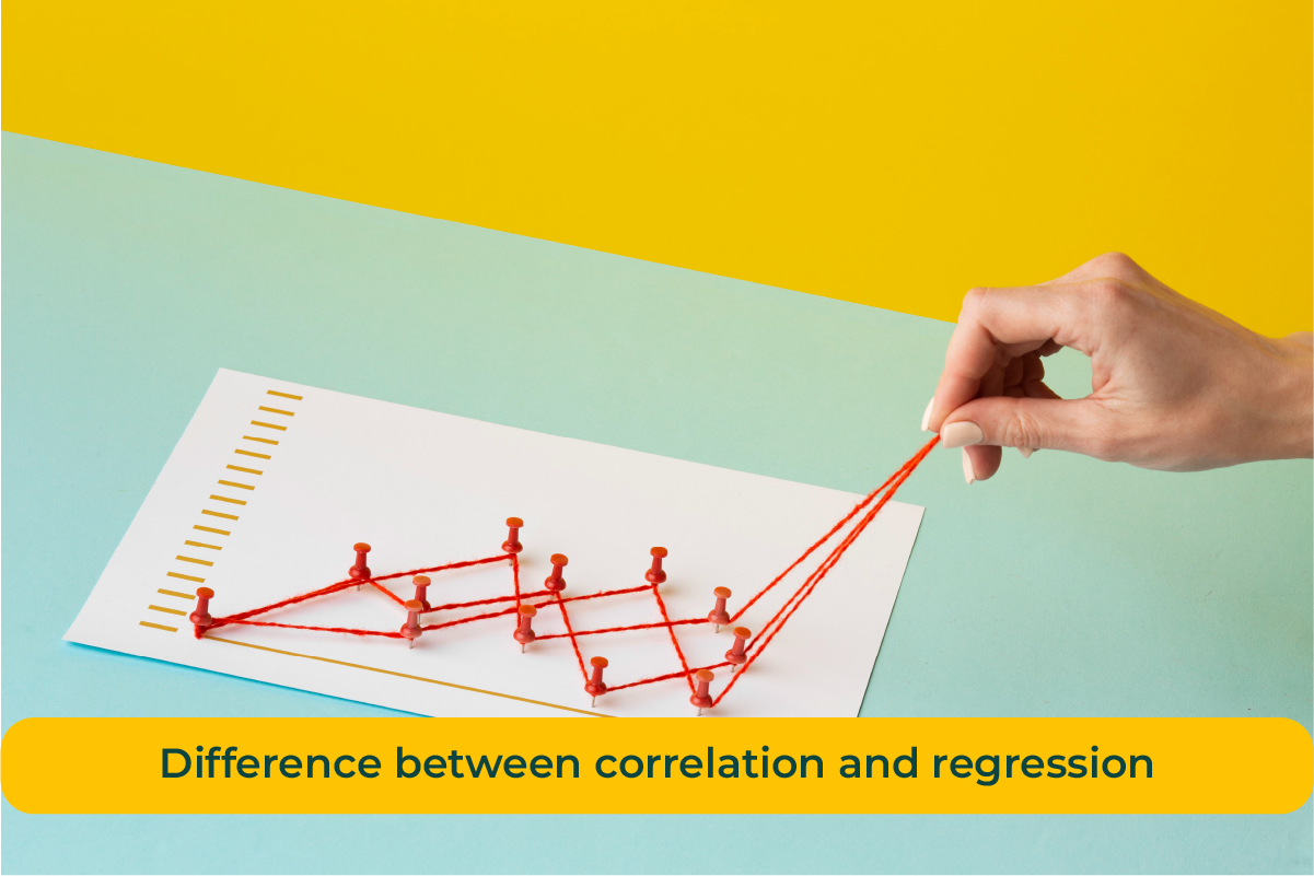
Hence, in this article, you will get an idea about the concept of correlation and regressions and how you can distinguish both based on several factors.

Introduction to Correlation

Correlation can be defined as a technique used in data statistics to come up with a relationship between any two or greater units of information. It is likewise used for forecasting weather.

The correlation coefficient which ranges from -1 to 0 to +1 is a relative indicator between two or more phenomena. A value of 1 tells us the two things are totally in perfect relationship with each other, a value of -1 indicates a total opposite situation of the other variable and a null value indicates no relationship between the two variables.

Types of Correlation

Positive Correlation

When both variables show a value or trend in the same direction it is called a positive correlation. If one of them is increasing, the second is increasing as well. For example, the relationship between examination rankings and the hours spent studying is regularly undoubtedly correlated.

Negative Correlation

A negative correlation exists when one variable increases while the other variable decreases. For instance, heating expenses and temperature levels have a negative correlation. As the temperature goes up the heating expenses seem to fall.

No Correlation

No correlation emerges when no relationship exists between two or more variables compared. For example, intelligence quotient and shoe size show little or no relationship If you increase or decrease one variable the other will not change.

Also Read: Data Analyst Interview Questions

Pearson’s Correlation Formula

The Pearson correlation coefficient (called r) is a statistic used to define the affiliation between two variables in terms of strength and direction. This is the formula that is used even when calculating Pearson’s correlation coefficient:

r = [n(Σxy) - (Σx)(Σy)] / sqrt{[n(Σx^2) - (Σx)^2] [n(Σy^2) - (Σy)^2]}

Breakdown of the formula

r: Pearson’s correlation coefficient.
n: The number of data points (or pairs of scores).
Σxy: The sum of the product of paired scores.
Σx: The sum of the x values.
Σy: The sum of the y values.
Σx²: The sum of the squared x values.
Σy²: The sum of the squared y values.

This formula calculates how closely two variables are related by comparing the product of their differences from the mean. The value of r can range from -1 to 1, where:

r = 1: Perfect positive linear relationship.
r = -1: Perfect negative linear relationship.
r = 0: No linear relationship.

Example Code in Python

Here’s a Python code that calculates Pearson’s correlation coefficient using two variables:

import numpy as np

# Example data

x = [10, 12, 13, 16, 18, 20]

y = [15, 18, 22, 24, 29, 33]

# Function to calculate Pearson correlation coefficient

def pearson_correlation(x, y):

n = len(x)  # Number of data points

sum_x = sum(x)  # Sum of x values

sum_y = sum(y)  # Sum of y values

sum_x_square = sum([i**2 for i in x])  # Sum of x^2 values

sum_y_square = sum([i**2 for i in y])  # Sum of y^2 values

sum_xy = sum([x[i] * y[i] for i in range(n)])  # Sum of x * y

# Calculate the Pearson correlation coefficient (r)

numerator = n * sum_xy - (sum_x * sum_y)

denominator = np.sqrt((n * sum_x_square - sum_x**2) * (n * sum_y_square - sum_y**2))

r = numerator / denominator

return r

# Calculate Pearson correlation for x and y

correlation = pearson_correlation(x, y)

print(f"Pearson correlation coefficient: {correlation:.3f}")

Explanation

Numerator = n * sum_xy – (sum_x * sum_y): The numerator of the Pearson formula calculates the covariance between the two datasets.
denominator: The denominator calculates the product of the standard deviations of both datasets.
r = numerator / denominator: The final step divides the numerator by the denominator to get the Pearson correlation coefficient.

Output

Pearson correlation coefficient: 0.990

In this example, the Pearson correlation coefficient is 0.990, which indicates a very strong positive linear relationship between the two variables.

Importance of Correlation in Data Analysis:

Data Simplification: It makes the diagnosis of complicated data easy by describing the interaction of two variables instead of making an examination of the whole data set.
Predictive Analysis: Predictive analysis relies on strong relationships with one variable to ascertain another which is likely to change within the course of the study.
Informs Decision Making: The relationship between two variables also aids in making useful decisions for businesses and research by finding patterns and relations in data.
Establishes Relationships: Correlation is valuable in establishing relationships in two variables whereby one indicates if they are moving in the same direction or in the opposite direction.
Initial Data Exploration: It’s a fundamental concept used during the beginning phase of data analysis which helps to spot potential relationships for deeper analysis.
Detect Outliers: Unusual or inconsistent data points that don’t fit the correlation pattern can be flagged as outliers for further investigation.

Real-time Applications of Correlation:

Finance: It is utilized to quantify market risk as the impact of stock prices on an index of stock market capitalization is examined.
Health care: This approach is used in relating the effects of any factors such as exercise and diet on a human being’s health.
Marketing: Through correlation, marketers analyze the Advertising Spend to Sales Growth relationship to budget and allocate.
Education: It is useful in finding the relationship between study habits and the class performance of students. It helps teachers to find successful strategies to teach students.
Economics: Correlation is applied to assess the relationship between unemployment rates and economic growth, influencing policy decisions.

Introduction to Regression

Regression is a statistical approach that allows for the evaluation of the relationship between a given variable called the dependent variable and other variables called independent variables in certain relations. This is useful because it enables one to find the value of the dependent variable even when certain values of the independent variables are already known. The regression model is commonly used in many applications where forecasting, trend-seeking, and decision-making are based on data.

Types of Regression with Formula and Examples

Linear Regression

Linear regression is said to linearize association between two variables combining any statistical data by the simplest method of making a curve through the data points. It is indicated by the formula:

Y = a + bX

Where:

Y: The dependent variable (predicted outcome)
X: The independent variable (input)
a: The intercept (where the line crosses the Y-axis)
b: The slope (the change in Y for a unit change in X)

Example:

This example shows predicting housing prices based on square footage. If bigger houses tend to have higher prices, a linear regression model can predict the price of a house based on its size.

# Import required libraries

import numpy as np

import matplotlib.pyplot as plt

from sklearn.linear_model import LinearRegression

# Example data: X represents independent variable (e.g., house size in square feet)

# Y represents dependent variable (e.g., house price)

X = np.array([600, 800, 1000, 1200, 1400]).reshape(-1, 1)  # Reshape for sklearn compatibility

Y = np.array([200, 250, 300, 350, 400])

# Create a Linear Regression model

model = LinearRegression()

# Train the model (fit the data)

model.fit(X, Y)

# Make predictions using the model

predicted_Y = model.predict(X)

# Output the model parameters

print(f"Intercept (a): {model.intercept_}")

print(f"Slope (b): {model.coef_[0]}")

# Predict the price of a house with 1600 square feet

predicted_price = model.predict([[1600]])

print(f"Predicted price for a 1600 sq ft house: {predicted_price[0]}")

# Plot the regression line with the data points

plt.scatter(X, Y, color='blue', label='Actual data')

plt.plot(X, predicted_Y, color='red', label='Regression line')

plt.xlabel('House Size (sq ft)')

plt.ylabel('House Price ($1000s)')

plt.title('Simple Linear Regression Example')

plt.legend()

plt.show()

Explanation:

X: The independent variable (house size in square feet).
Y: The dependent variable (house price in thousands).
The model is trained to find the best-fit line. The slope (b = 0.25) tells us that for every additional square foot, the house price increases by 0.25 (or $250).
The intercept (a = 100) means if the house size were 0, the predicted price would start at $100,000.
It predicts the price of a 1600-square-foot house as $500,000.

Output:

Intercept (a): 100.0

Slope (b): 0.25

Predicted price for a 1600 sq ft house: 500.0

Multiple Linear Regression

This is an extension of linear regression where more than one independent variable is used to predict the dependent variable. The formula is:

Y = a + b1X1 + b2X2 + … + bnXn

Where:

Y: The dependent variable
X1, X2, …, Xn: The independent variables
b1, b2, …, bn: Coefficients that represent the impact of each independent variable on Y

Logistic Regression

Logistic regression is used when the dependent variable is binary (e.g., 0 or 1, yes or no). It predicts the probability of an event occurring. The formula is:

P(Y=1) = 1 / (1 + e^-(a + bX))

Where:

P(Y=1): The probability of the dependent variable being 1
e: Euler’s number (a constant)
a: The intercept
b: The coefficient for the independent variable

Importance of Regression

Predictive Power: By employing Regression, the future value of any consistent data can easily be obtained which is very helpful when forecasting for the business.
Understanding Relationships: It describes how independent variable change modifies the unit area, which assists in establishing the cause-and-effect relationship.
Evaluating Ways: Companies also employ regression strategies for evaluating other strategies, such as finding out what factors influence sales or performance improvement the most.

Applications of Regression

Finance: To forecast stock prices by examining historical data and factors affecting the market.
Healthcare: A highly specialised area where algorithms churn out accurate prognoses on diseases by factoring in patient risk factors like age, weight, and other prevalent health characteristics.
Marketing: Helps in measuring the effectiveness of advertisements on the market sales and helps companies make wise budgetary allocations.
Economics: The regression is also used by economists to analyse the effect of certain variables like inflation or interest on GDP changes.

Difference Between Correlation and Regression

Aspect	Correlation	Regression
Definition	Measures the strength and direction of a relationship between two variables.	Predicts the value of one variable based on the known value(s) of another variable(s).
Purpose	To determine whether and how strongly variables are related.	To model and predict relationships between dependent and independent variables.
Types	Pearson, Spearman Rank, Kendall Tau	Linear, Multiple Linear, Logistic
Independent & Dependent	No distinction between independent and dependent variables.	Distinguishes between dependent (predicted) and independent (predictor) variables.
Nature of Relationship	Measures the degree of association (how variables move together).	Establishes a cause-and-effect relationship.
Usage	To find associations or correlations between variables.	To predict the value of the dependent variable.
Equation	No specific equation (correlation coefficient is calculated).	Regression equations (e.g., Y = a + bX for linear regression).
Range of Values	Correlation coefficient (r) ranges from -1 to +1.	No range; the dependent variable is predicted based on independent variables.
Assumptions	Assumes only a linear relationship (in Pearson correlation).	Assumes a specific form of relationship (linear, polynomial, etc.).
Causality	Does not imply causality.	Can suggest causality if certain assumptions are met.

Similarities Between Correlation and Regression

Both Analyze Relationships: In both correlation and regression, the study is centred on the relationship between two or more parameters. Whereas correlation is concerned with measuring the strength and the direction between two or more variables, regression predicts quantitative outcomes based on the relationship.
Based on Quantitative Data: Both techniques require numerical data for the variables being analysed. Whether it’s height and weight or sales and marketing spend, both methods work with continuous or ordinal data.
Statistical Tools: In the scientific fields, it is common to employ both correlation and regression as they are analytical methods that are often applied and useful to data, research, and forecasts. The methods are useful in determining the interactions among the variables and the variables and making decisions based on the collected data.
Involve Calculations: Both methods involve mathematical calculations, using formulas to find specific values (e.g., correlation coefficient for correlation, regression coefficients for regression). These values then provide insights into the data’s relationship.
Require Data Pairs: In the case of both methods, data is obtained in pairs. Correlation studies the extent two variables are related whereas the regression analysis predicts one variable through the other(s) by modelling them according to their relation obtained through correlation.
Linear Relationships: Pearson correlation and simple linear regression are two techniques that can be employed with the assumption of linear relationships between the variables. Other relationships can also be examined using different techniques such as Spearman correlation and polynomial regression.

Conclusion

To sum up, correlation and regression are two major statistical approaches towards the interpretation of relationships between different variables. While correlation is all about how close a relationship is and its direction, regression aims at determining the value of one variable through the knowledge of another variable. Each of these techniques has its own specific applications in various scenarios and performs an invaluable role in engaging data.

Being aware of the differences and similarities between different methods enables you to select the best one for your analytical task. It does not matter whether you have to seek relationships or forecast data: both correlation and regression broaden the horizon of data and enable you to utilise it efficiently. Are you an aspiring data scientist? Consider pursuing Hero Vired’s Advanced Certification Program in Data Science & Analytics powered by the University of Chicago.